Inverse scattering transform
In mathematics, the inverse scattering transform is a method for solving some non-linear partial differential equations. It is one of the most important developments in mathematical physics in the past 40 years. The method is a non-linear analogue of the Fourier transform, which itself can be applied to solve many linear partial differential equations.
The inverse scattering transform may be applied to many of the so-called exactly solvable models, that is to say completely integrable infinite dimensional systems. These include the Korteweg–de Vries equation, the nonlinear Schrödinger equation, the coupled nonlinear Schrödinger equations, the Sine-Gordon equation, the Kadomtsev–Petviashvili equation, the Toda lattice equation, the Ishimori equation, the Dym equation etc. A further, particularly interesting, family of examples is provided by the Bogomolny equations (for a given gauge group and oriented Riemannian 3-fold), the  solutions of which are magnetic monopoles.
A characteristic of solutions obtained by the inverse scattering method is the existence of solitons which have no analogue for linear partial differential equations. The term "soliton" arises from non-linear optics.
The inverse scattering problem can be written as a Riemann–Hilbert factorization problem. This formulation can be generalized to differential operators of order greater than 2 and also to periodic potentials.
Contents |
Example: the Korteweg–de Vries equation
The Korteweg–de Vries equation is a nonlinear, dispersive, evolution partial differential equation for a function u; of two real variables, one space variable x and one time variable t :
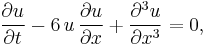
with  and
and  denoting partial derivatives with respect to t and x.
To solve the initial value problem for this equation where  is a known function of x, one associates to this equation the Schrödinger eigenvalue equation
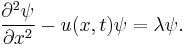
where  is an unknown function of t and x and u is the solution of the Korteweg–de Vries equation that is unknown except at
  . The constant
  is an eigenvalue.
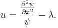
From the Schrödinger equation we obtain
Substituting this into the Korteweg–de Vries equation and integrating gives the equation
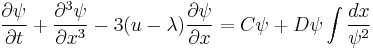
where C and D are constants.
Method of solution
Step 1. Determine the nonlinear partial differential equation. This is usually accomplished by analyzing the physics of the situation being studied.
Step 2. Employ forward scattering. This consists in finding the Lax pair. The Lax pair consists of two linear operators,  and
and  , such that
  and
and  , where the subscript t in
  denotes the time derivative of
  . It is extremely important that the eigenvalue be independent of time; i.e.
  Necessary and sufficient conditions for this to occur are determined as follows: take the time derivative of to obtain
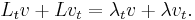
Plugging in  for yields

Rearranging on the far right term gives us

Thus,

Since  , this implies that
  if and only if
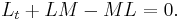
This is Lax's equation. One important thing to note about Lax's equation is that  is the time derivative of precisely where it explicitly depends on
  . The reason for defining the differentiation this way is motivated by the simplest instance of , which is the Schrödinger operator (see Schrödinger equation):
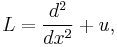
where u is the "potential". Comparing the expression  with
with 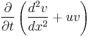 shows us that
  thus ignoring the first term.
After concocting the appropriate Lax pair it should be the case that Lax's equation recovers the original nonlinear PDE.
Step 3. Determine the time evolution of the eigenfunctions associated to each eigenvalue , the norming constants, and the reflection coefficient, all three comprising the so-called scattering data. This time evolution is given by a system of linear ordinary differential equations which can be solved.
Step 4. Perform the inverse scattering procedure by solving the Gelfand–Levitan–Marchenko integral equation (Israel Moiseevich Gelfand and Boris Moiseevich Levitan;[1] Vladimir Aleksandrovich Marchenko[2]), a linear integral equation, to obtain the final solution of the original nonlinear PDE. All the scattering data is required in order to do this. Note that if the reflection coefficient is zero, the process becomes much easier. Note also that this step works if is a differential or difference operator of order two, but not necessarily for higher orders. In all cases however, the inverse scattering problem is reducible to a Riemann–Hilbert factorization problem. (See Ablowitz-Clarkson (1991) for either approach. See Marchenko (1986) for a mathematical rigorous treatment.)
List of integrable equations
- Korteweg–de Vries equation
- nonlinear Schrödinger equation
- Camassa-Holm equation
- Sine-Gordon equation
- Toda lattice
- Ishimori equation
- Dym equation and so on.
References
- M. Ablowitz, H. Segur, Solitons and the Inverse Scattering Transform, SIAM, Philadelphia, 1981.
- N. Asano, Y. Kato, Algebraic and Spectral Methods for Nonlinear Wave Equations, Longman Scientific & Technical, Essex, England, 1990.
- M. Ablowitz, P. Clarkson, Solitons, Nonlinear Evolution Equations and Inverse Scattering, Cambridge University Press, Cambridge, 1991.
- V. A. Marchenko, "Sturm-Liouville Operators and Applications", Birkhäuser, Basel, 1986.
- J. Shaw, Mathematical Principles of Optical Fiber Communications, SIAM, Philadelphia, 2004.
- Eds: R.K. Bullough, P.J. Caudrey. "Solitons" Topics in Current Physics 17. Springer Verlag, Berlin-Heidelberg-New York, 1980.